Steepest Descent II: The Local Central Limit Theorem

August 6, 2026 · math, random matrix theory

Introduction

In Steepest Descent I we introduced Laplace’s method (the real integral version) and used it to prove Stirling’s formula. There, all we needed to do was localize near the maximum of $f$. In this post, we do proper steepest descent, which becomes significantly more complicated as you have to choose a contour. This was the second example in Vadim Gorin’s course, but treated with substantially more rigor.

The general formula in $\CC$ we wrote down but didn’t yet need is

The complication is that $\gamma$ is now a contour we have to choose. On a bad contour, $e^{nf(z)}$ oscillates instead of decaying, and Laplace’s argument falls apart. The method is called “steepest descent” because we choose a contour such that $\Re f$ decreases as fast as possible away from $z_0$ and does not oscillate. We take $\gamma$ through the critical point $z_0$ along the direction where $\Im f$ stays constant so there is no oscillation and $\Re f$ decays. We will prove the local central limit theorem using steepest descent and walk through the construction of such a contour.

So, the steps are similar to those in Steepest Descent I, but with the addition of choosing a contour.

1. Express the desired formula as an integral.
2. Find an adequate $f$ to to transform the integrand into $\exp(nf(z))$.
3. Find an appropriate contour.
4. Localize near the critical point of $f$ with only $o(1)$ loss.
5. Bound the tails.

Local CLT for Binomial Random Variables

Theorem (Local Central Limit Theorem). Let $p \in (0,1)$ and $x \in \RR$. For $n \in \ZZ_+$, let $k$ be the nearest integer to $pn + x\sqrt{n}$. Then

This theorem predates the more familiar Central Limit Theorem — De Moivre proved it for $p=1/2$, and Laplace in general. It says something sharper than the CLT: not just that a properly-normalized binomial random variable converges in distribution to a Gaussian, but that its individual point masses converge to the values of the Gaussian density itself, at scale $n^{-1/2}$. Hence “local.”

Proof.

Step 1: We observe that $p^k(1-p)^{n-k}{n \choose k}$ is the coefficient of $z^k$ in

Dividing by $z^{k+1}$ turns this into the coefficient of $z^{-1}$, i.e. a residue, and the Residue Theorem lets us write it as a contour integral around $0$:

We recast this as

where $f(z) = \log(pz + (1 - p)) - p \log(z)$. We’ll treat $z^{np-k-1}$ separately — its exponent grows only like $O(\sqrt{n})$, far slower than the $nf(z)$ term that will dominate everything.

Step 2: As with Laplace’s method, we want to localize near a critical point of $f$. But we’re now integrating over a closed contour in $\CC$ rather than an interval in $\RR$, so we also have to choose that contour, and worry about the geometry and oscillation of the integrand along it. We first fix a branch of $\log$: cut along the negative real axis, so $\log(re^{\ii\theta}) = \log r + \ii\theta$ for $\theta \in (-\pi,\pi)$.

which vanishes exactly when $p(1-p)(z-1) = 0$, i.e. at $z_c = 1$. Furthermore,

Since $f(1) = \log(1) - p\log(1) = 0$, Taylor expanding gives

Because $f$ is holomorphic, the Cauchy–Riemann equations force this critical point to be a saddle: $f’‘(z_c)$ is real and positive, so $\Re f$ falls off in the imaginary direction and rises in the real direction near $z_c$. The figure below shows the local picture.

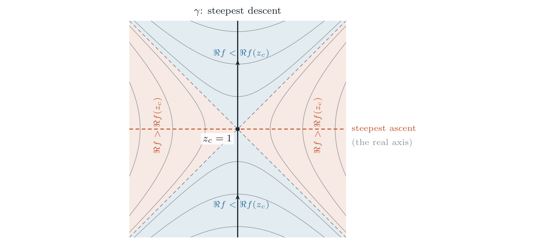
Step 3: We want a contour through $z_c=1$ on which $\Im f$ stays constant (so the integrand doesn’t oscillate) and $\Re f$ is maximized at $z_c$ (so Laplace’s argument applies once we’re on it). Consider the level set $\Im f(z) = \Im f(z_c) = 0$. The positive real ray $(0,\infty)$ trivially lies in it, since $f$ is real there, but we claim it also contains a loop around $0$, which we’ll take as our contour.

$\Im f(z) = 0$ is equivalent to $g(z) := (pz + (1 - p))z^{-p} \in (0, \infty)$, a form that’s easier to work with. Writing $z = re^{\ii \theta}$,

so

Setting $\Im g(z) = 0$ (and $r^{-p}\ne 0$) requires the two terms to balance:

At $\theta=0$ both sides vanish trivially which is the ray we already found. For $\theta \ne 0$: since $\theta \in (-\pi,\pi)$ forces $(1-p)\theta \in (-\pi,\pi)$ too, $\sin((1-p)\theta) \ne 0$, so we can solve for $r$:

$R(\theta) > 0$ for all $\theta$, so $\gamma(\theta) = R(\theta)e^{\ii \theta}$ is injective and winds once around $0$, and $R(0)=1$ (by L’Hôpital), so $\gamma$ passes through $z_c$ exactly as required. The figure below draws $\gamma$ for a few values of $p$.

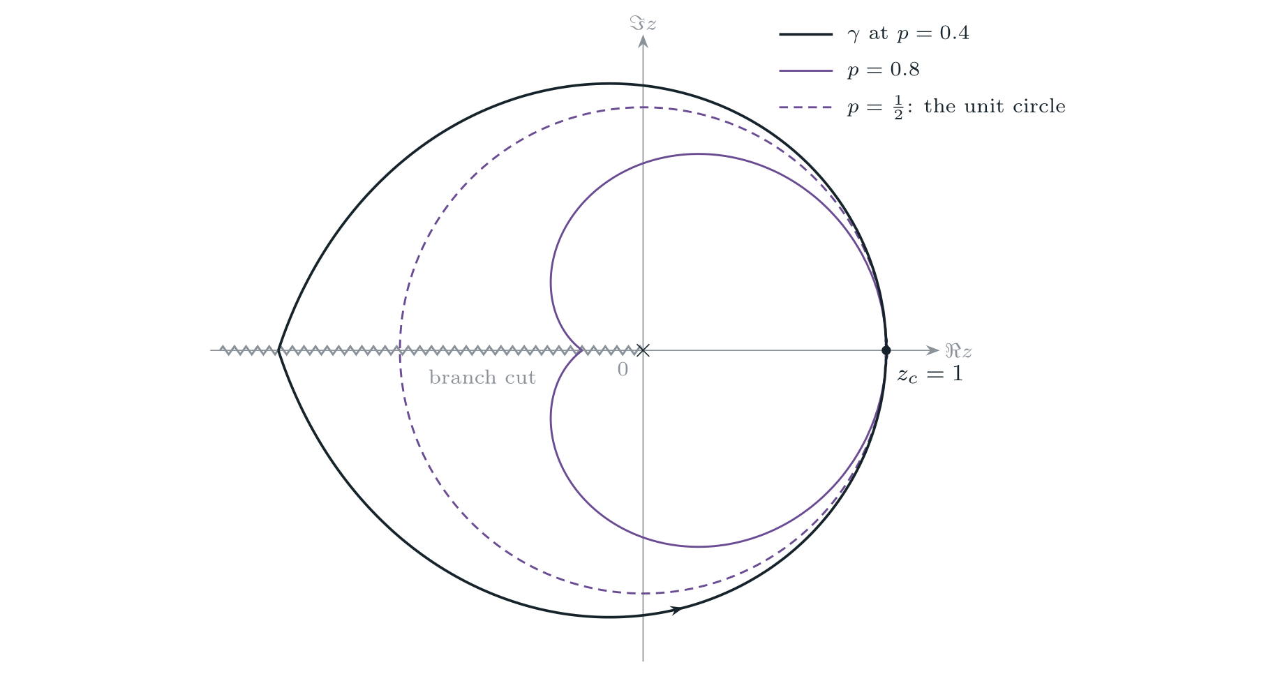
It remains to check $\Re g$ (i.e. $g$ itself, since it’s real on $\gamma$) is positive rather than negative there. Substituting $r=R(\theta)$ and using the sine addition formula $\sin(p\theta)\cos((1-p)\theta) + \cos(p\theta)\sin((1-p)\theta) = \sin\theta$,

which is positive because $\sin\theta$ and $\sin((1-p)\theta)$ always share a sign for $\lvert\theta\rvert<\pi$. So $\gamma(\theta)$ genuinely lies in ${\Im f = 0}$.

We appeal to a general fact: along a level set of $\Im f$, $\Re f$ is monotonic. Write $f = u + \ii v$ with $z = x+\ii y$. The Cauchy–Riemann equations $u_x = v_y$, $u_y=-v_x$ give $\nabla v = (-u_y, u_x)$, so $\nabla u \cdot \nabla v = 0$ and $\lvert\nabla u\rvert = \lvert\nabla v\rvert = \lvert f’\rvert$. The tangent to a level curve of $v$ is orthogonal to $\nabla v$, hence parallel to $\nabla u$, so along $\gamma$,

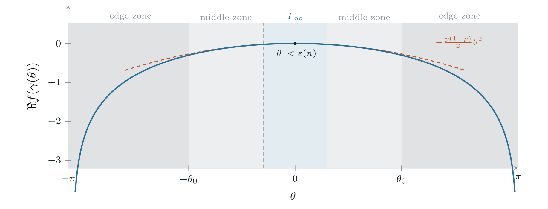
which is nonzero away from the critical point. So $\Re f$ is monotonic on $(-\pi,0)$ and on $(0,\pi)$ separately. Since $\Re f(\gamma(\theta)) \to -\infty$ as $\theta \to \pm\pi$ (the pinch point from Step 3), $\Re f$ must rise from $-\infty$ up to $\theta=0$ and fall back to $-\infty$ past it. $\Re f$ attains its maximum exactly at $z_c$. The figure below plots this profile, together with the zones we’ll use to bound the tail below.

Step 4: Write $u(\theta) = f(\gamma(\theta))$. Since $f(1)=0$, $f’(1)=0$, $f’‘(1) = p(1-p)$, and $\gamma’(0) = (R’(0)+\ii R(0))e^{\ii \cdot 0} = \ii$ (using that $R$ is even since it’s a ratio of two odd functions, so $R’(0)=0$), we have $\gamma(\theta) = 1+\ii\theta + O(\theta^2)$ and

As in the Stirling proof, we split at $\vep(n) = n^{-2/5}$ — the same balance survives unchanged, since the error term here is cubic exactly as it was there. Write $I(n) = I_{\mathrm{loc}}(n) + I_{\mathrm{tail}}(n)$, the integral \eqref{eq:clt_int} restricted to $\lvert\theta\rvert<\vep(n)$ and its complement.

For $I_{\mathrm{loc}}$, substitute $t = \theta\sqrt{n}$, so $\lvert t\rvert < \sqrt{n}\,\vep(n) = n^{1/10}$. Equation \eqref{eq:clt_u_taylor} gives

and, writing $np-k-1 = -x\sqrt{n} + \delta_n$ with $\lvert\delta_n\rvert<2$ (from the choice of $k$) and $\log\gamma(\theta) = \log R(\theta) + \ii \theta$,

while the Jacobian is $\gamma’(t/\sqrt{n}) = \ii(1+O(n^{-2/5}))$. Together,

Extending the domain of integration to all of $\RR$ costs $O\lp e^{-p(1-p)n^{1/5}/2} \rp$, and evaluating the Fourier transform of the resulting Gaussian,

Step 5: For the tail, uniformly bound the Jacobian $\lvert\gamma’(\theta)\rvert \le M$ (continuous on a compact set), and set $F(n,\theta) = nu(\theta) + (np-k-1)\log R(\theta)$, so

In the middle zone $\vep(n)<\lvert\theta\rvert<\theta_0$, \eqref{eq:clt_u_taylor} gives $u(\theta) < -\tfrac{p(1-p)}{4}\theta^2$, and since $\lvert\log R(\theta)\rvert \le C_1\theta^2$ and $\lvert np-k-1\rvert \le (\lvert x\rvert+1)\sqrt{n}$, for $n$ sufficiently large

so, using $\theta^2 \ge \vep(n)^2 = n^{-4/5}$ on this range,

In the edge zone $\theta_0 < \lvert\theta\rvert < \pi$, there is $c<0$ with $u(\theta) < c$, and $R(\theta)$ is bounded away from $0$ and $\infty$, so $\lvert\log R(\theta)\rvert \le C_2$. Hence $F(n,\theta) \le cn + C_2(\lvert x\rvert+1)\sqrt{n} \le \tfrac{c}{2}n$ for $n$ large, and

Both bounds decay faster than any power of $n$, so absorbing constants and prefactors into a single $c^*>0$,

Combining with \eqref{eq:clt_center}, whose leading term is already $\Theta(n^{-1/2})$, the tail is absorbed into the multiplicative error and

which is exactly \eqref{eq:local_clt}. $\blacksquare$